Trees

A tree is a hierarchical data structure consisting of a set of connected nodes where:

Each node may have multiple other nodes as children (depending on the type of tree)

Each node is connected to one parent except the root node

A binary tree is a tree where each node can have up to two child nodes, referred to as the left child and the right child.

Binary Search Trees

A binary search tree is an ordered binary tree, where for each node:

• All values in the left subtree are less than the value in the node
• All values in the right subtree are greater than the value in the node

Terminologies

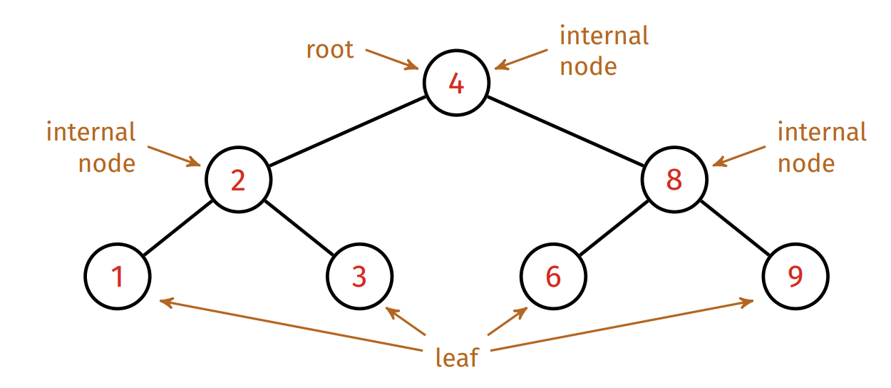
The root node is the node with no parent node.

A leaf node is a node that has no child nodes.

An internal node is a node that has at least one child node.

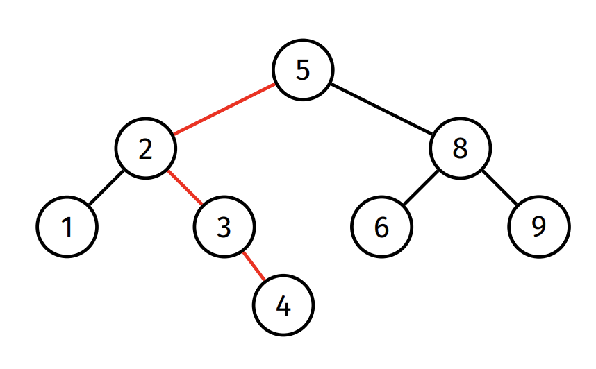
Height of a tree: Maximum path length from the root node to a leaf

• The height of an empty tree is considered to be -1
• The height of the following tree is 3

For a tree with $n$ nodes:

• The maximum possible height is $n − 1$
• The minimum possible height is $\lfloor \log_2 n \rfloor$

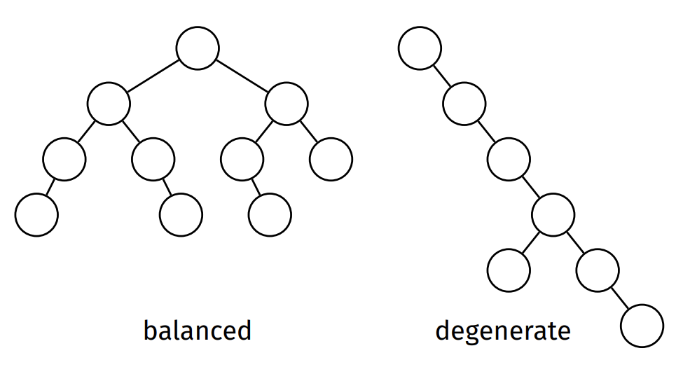
For a given number of nodes, a tree is said to be

• balanced if its height is minimal (or close to minimal), and
• degenerate if its height is maximal (or close to maximal).

BST Operations

The height $h$ of a binary search tree determines the efficiency of many operations, so we will use both $n$ and $h$ in our analyses.

Insertion

Insertion method:

• Start at the root
• Compare value to be inserted with value in the node
  • If value being inserted is less, descend to left child
  • If value being inserted is greater, descend to right child
• Repeat until you have to go left/right but current node has no left/right child
  • Create new node and attach to current node

Analysis:

• At most one node is visited per level
• Number of operations performed per node is constant
• Therefore, the worst-case time complexity of insertion is $O(h)$ where $h$ is the height of the BST

Search

Given a BST $t$ and a value $v$, return true if $v$ is in the BST and false otherwise

Method is similar to insertion, except we don’t create a new node.

Analysis:

• At most one node is visited per level
• Number of operations performed per node is constant
• Therefore, the worst-case time complexity of search is $O(h)$ where $h$ is the height of the BST

Traversal

There are 4 common ways to traverse a binary tree:

1. Pre-order (NLR):

• visit root, then traverse left subtree, then traverse right subtree
• Useful for reconstructing a tree

2. In-order (LNR):

• traverse left subtree, then visit root, then traverse right subtree
• Useful for traversing a BST in ascending order

3. Post-order (LRN):

• traverse left subtree, then traverse right subtree, then visit root
• Useful for evaluating an expression tree
• Useful for freeing a tree

4. Level-order:

• visit root, then its children, then their children, and so on
• Useful for printing a tree

Analysis:

• Each node is visited once
• Hence, time complexity of tree traversal is O(n), where n is the number of nodes

Level order traversal pseudocode:

Level Order Traversal(BST t):
  initialise an empty queue
  add t's root node to the queue
  while the queue is not empty do
    remove node x from the front of the queue
    print the value in x
    add the left child (if any) of x to the queue
    add the right child (if any) of x to the queue
  end while

P.S. level order traversal can be seen as a BFS

Join

Given two BSTs $t_1$ and $t_2$ where max($t_1$) < min($t_2$), return a BST containing all items from $t_1$ and $t_2$

Method:

1. Find the minimum node $min$ in $t_2$
2. Replace $min$ by its right subtree (if it exists)
3. Elevate $min$ to be the new root of $t_1$ and $t_2$

Analysis:

• The join algorithm simply finds the minimum node in $t_2$
• Thus, at most one node is visited per level of $t_2$
• Therefore, the worst-case time complexity of join is $O(h_2)$ where $h_2$ is the height of $t_2$

Deletion

Given a BST $t$ and a value $v$, delete $v$ from the BST, and return the root of the updated BST

Recursive method:

• $t$ is empty:
  • result is empty
• $v < t$->item
  • delete $v$ from $t$’s left subtree
• $v > t$->item
  • delete $v$ from $t$’s right subtree
• v = t->item
  • three sub-cases:
    • t is a leaf ⇒ result is empty tree
    • t has one subtree ⇒ replace with subtree
    • t has two subtrees ⇒ join the two subtrees

Analysis:

• The deletion algorithm traverses down just one branch
  • First, the item being deleted is found
  • If the item exists and has two subtrees, its successor is found
• Thus, at most one node is visited per level
• Therefore, the worst-case time complexity of deletion is $O(h)$ where $h$ is the height of the BST

Balance

Types of balance:

• Size-balance
  • a size-balanced tree has, for every node, |size($l$) - size($r$)| $\leq$ 1
• Height-balance
  • a Height-balanced tree has, for every node, |height($l$) - height($r$)| $\leq$ 1

Balancing Operations

Rotation

• Left rotation
• Right rotation

struct node *rotateRight(struct node *root) {
  if (root == NULL || root->left == NULL) return root;
  struct node *newRoot = root->left;
  root->left = newRoot->right;
  newRoot->right = root;
  return newRoot;
}

struct node *rotateLeft(struct node *root) {
  if (root == NULL || root->right == NULL) return root;
  struct node *newRoot = root->right;
  root->right = newRoot->left;
  newRoot->left = root;
  return newRoot;
}

Time complexity: O(1)

• Rotation requires only a few localised pointer re-arrangements

Partition

Rearrange the tree so that the element with index $i$ becomes the root

Method:

• Find element with index $i$
• Perform rotations to lift it to the root
  • If it is the left child of its parent, perform right rotation at its parent
  • If it is the right child of its parent, perform left rotation at its parent
  • Repeat until it is at the root of the tree

partition(t, i):
  Input: tree t, index i
  Output: tree with i-th item moved to root

  leftSize = size(t->left)

  if i < leftSize:
    t->left = partition(t->left, i)
    t = rotateRight(t)
  else if i > leftSize:
    t->right = partition(t->right, i - leftSize - 1)
    t = rotateLeft(t)
  return t

Analysis:

• size() operation is expensive
• Can cause partition to be $O(n^2)$ in the worst case
• To improve efficiency, can change node structure so that each node stores the size of its subtree in the node itself
  • However, this will require extra work in other functions to maintain

struct node {
    int item;
    struct node *left;
    struct node *right;
    int size;
};

Balancing Methods

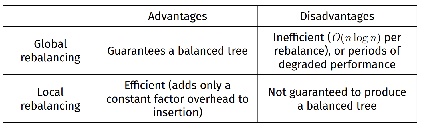
Global Rebalancing

Completely rebalance whole tree so it is size-balanced

Method:

• Lift the median node to the root by partitioning on index size(t)/2
• rebalance both subtrees (recursively)

rebalance(t):
  Input: tree t
  Output: rebalanced t

  if size(t) < 3:
    return t

  t = partition(t, size(t) / 2)
  t->left = rebalance(t->left)
  t->right = rebalance(t->right)
  return t

Worst-case time complexity: $O(n \log n)$

• Assume nodes store the size of their subtrees
• First step: partition entire tree on index $n/2$
  • This takes at most $n$ recursive calls, $n$ rotations ⇒ $n$ steps
  • Result is two subtrees of size ≈ $n/2$
• Then partition both subtrees
  • Partitioning these subtrees takes $n/2$ steps each ⇒ $n$ steps in total
  • Result is four subtrees of size ≈ $n/4$
• …and so on…
• About $\log_2 n$ levels of partitioning in total, each requiring $n$ steps ⇒ $O(n \log n)$

Periodic Rebalancing:

bstInsert(t, v):
  Input: tree t, value v
  Output: t with v inserted

  t = insertAtLeaf(t, v)

  if size(t) mod k = 0:
    t = rebalance(t)
  
  return t

• Good if tree is not modified very often
• Otherwise…
  • Insertion will be slow occasionally due to rebalancing
  • Performance will gradually degrade until next rebalance

Local Rebalancing

Perform small, efficient, localised operations in an attempt to improve the overall balance of the tree

Root Insertion

Insert new value normally (at the leaf) and then rotate the new node up to the root.

insertAtRoot(t, v):
  Input: tree t, value v
  Output: t with v inserted at the root

  if t is empty:
    return new node containing v
  else if v < t->item:
    t->left = insertAtRoot(t->left, v)
    t = rotateRight(t)
  else if v > t->item:
    t->right = insertAtRoot(t->right, v)
    t = rotateLeft(t)

  return t

Analysis:

• Same time complexity as normal insertion: $O(h)$
• Tree is more likely to be balanced, but no guarantee
• Root insertion ensures recently inserted items are close to the root
  • Useful for applications where recently added items are more likely to be searched
• Major problem: ascending-ordered and descending-ordered data is still a worst case for root insertion

Randomised Insertion

Introduce some randomness into insertion algorithm:

• Randomly choose whether to insert normally or insert at root

insertRandom(t, v):
  Input: tree t, value v
  Output: t with v inserted
  if t is empty:
    return new node containing v

  // p/q chance of inserting at root
  if random() mod q < p:
    return insertAtRoot(t, v)
  else:
    return insertAtLeaf(t, v)

Randomised insertion creates similar results to inserting items in random order.

Tree is more likely to be balanced (but no guarantee)

Summary

AVL Trees

Method:

• Insert item recursively
• Check balance at each node along the insertion path in reverse
  • i.e., from bottom to top
• Fix imbalances as they are found

Since AVL trees are always height-balanced, the height of an AVL tree is guaranteed to be at most $\log n$

Insertion

Insertion process:

1. if the tree is empty:

• return new node

2. insert recursively
3. check (and fix) balance
4. return root of updated tree

There are 4 rebalancing cases:

1. Left Left

• bal(t) > 1 and bal(t->left) >= 0
• Rotate right at t

2. Left Right

• bal(t) > 1 and bal(t->left) < 0
• Rotate left at t->left, then rotate right at t

3. Right Left

• bal(t) < -1 and bal(t->right) > 0
• Rotate right at t->right, then rotate left at t

4. Right Right

• bal(t) < -1 and bal(t->right) <= 0
• Rotate left at t

Analysis:

• Height of an AVL tree is $O(\log n)$
• In the worst case, length of insertion path is $O(\log n)$
• Have to maintain height data and check/fix balance at each node on insertion path
  • This is $O(1)$ per node
• Therefore, worst-case time complexity of AVL tree insertion is $O(\log n)$

Search

Exactly the same as for regular BSTs.

Worst-case time complexity is $O(\log n)$, since AVL trees are height-balanced.

Deletion

Method:

• Delete item recursively
• Check balance at each node along the deletion path∗ in reverse
• Fix imbalances as they are found

Analysis:

• Height of an AVL tree is $O(\log n)$
• In the worst case, length of deletion path is $O(\log n)$
• Have to maintain height data and check/fix balance at each node on deletion path
  • This is $O(1)$ per node
• Therefore, worst-case time complexity of AVL tree deletion is $O(\log n)$

Summary

AVL trees are always height-balanced

• This means the height of an AVL tree is $O(\log n)$
• Rotations are used to fix imbalances during insertion and deletion
• Balance is checked efficiently by storing height data in each node, which needs to be maintained
• Worst-case time complexity of $O(\log n)$ for insertion, search and deletion
• Can be used to implent a set ADT efficiently with contains, insert, delete at $O(\log n)$