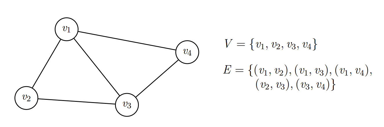
Graphs

Graph Basics

A graph is a data structure consisting of:

• A set of vertices $V$
  • Also called nodes
• A set of edges $E$ between pairs of vertices

Types of Graphs

• Undirected
  • In an undirected graph, edges do not have direction. For example, Facebook friends.
• Directed
  • In a directed graph or digraph, each edge has a direction. For example, road maps, Twitter follows.
• Weighed
  • In a weighted graph, each edge has an associated weight. For example, road maps, networks.
• With Loops
  • A loop is an edge from a vertex to itself. Depending on the context, a graph may or may not be able to have loops.
• Multigraphs
  • In a multigraph, multiple edges are allowed between two vertices. For example, call graphs, maps.

A simple graph is an undirected graph with no loops and no multiple edges.

For a simple graph with V vertices, the maximum possible number of edges is

$$E = V(V-1)/2$$

Graph Terminology

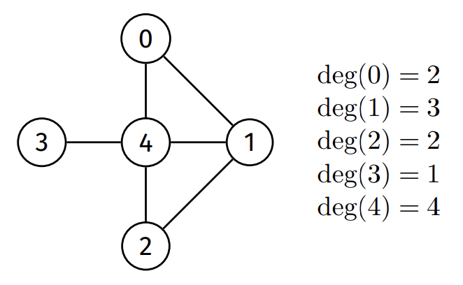
Two vertices $v$ and $w$ are adjacent if an edge $e := (v,w)$ connects them; we can $e$ is incident on $v$ and $w$.

The $degree$ of a vertex $v$ is the number of edges incident on $v$

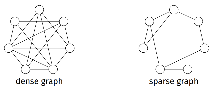
The ratio $E:V$ can vary considerably.

If $E$ is closer to $V^2$, the graph is dense.

If $E$ is closer to $V$, the graph is sparse.

A path is aa sequence of vertices where each vertex has an edge to the next in the sequence

A path is simple if it has no repeating vertices

A cycle is a path where only the first and last vertices are the same

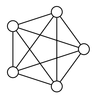
A complete graph is a graph where every vertex is connected to every other vertex via an edge.

In a complete graph, $E = \frac{1}{2}V(V-1)$

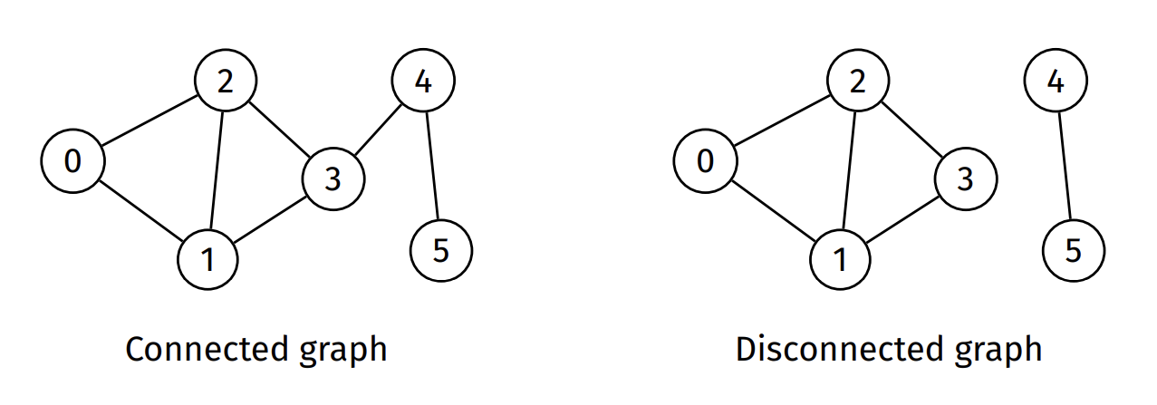
A connected graph is a graph where there is a path from every vertex to every other vertex

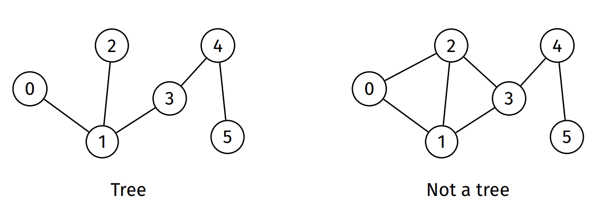
A tree is a connected graph with no cycles. A tree has exactly one path between each pair of vertices.

A subgraph of a graph G is a graph that contains a subset of the vertices of G and a subset of the edges between these vertices.

A connected component is a maximally connected subgraph. A connected graph has one connected component — the graph itself. A disconnected graph has two or more connected components.

A spanning tree of a graph G is a subgraph that contains all the vertices of G and is a single tree. Spanning trees only exist for connected graphs.

A spanning forest of a graph G is a subgraph that contains all the vertices of G and contains one tree for each connected component.

A clique is a complete subgraph. A clique is non-trivial if it has 3 or more vertices.

Graph Traversals

Graphs aren’t very useful if all we’re doing is storing data in them. We need to effectively search and traverse them to gather information.

There are three 3 main topics related to traversal:

1. Traverse for Item Searching
   • Move between nodes to look for a value
2. Traverse for Path Finding
   • Look for a value, but keep track on how to get there
3. Traverse Fully
   • Like path-finding but exploring the full graph

There are two primary methods to traverse a graph:

• Breadth-first search (BFS)
  • Iterative solutions
• Depth-first search (DFS)
  • Recursive & iterative solutions

Both approaches ignore some edges by remembering previously visited vertices, usually done in a visited[] array (this also prevents cycles).

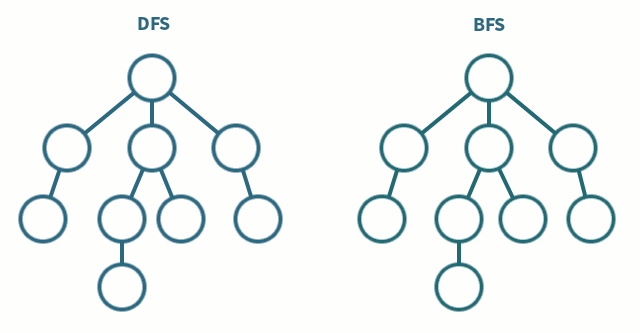
Breadth First Search

Start at a node, and expanding out equally from there. Visit all the neighbours of the current vertex, then visit all the neighbours of those neighbours, etc.

bfs(G, src):
  Input: graph G, starting vertex src

  create visited array, initialised to false
  create predecessor array, initialised to -1
  create queue Q

  visited[src] = true
  enqueue src into Q

  while Q is not empty:
    v = dequeue from Q
    for each neighbour w of v in G where visited[w] = false:
      visited[w] = true
      predecessor[w] = v
      enqueue w into Q

The previous code can be simplified:

• The predecessor array can double as a visited array.
• $predecessor[v] = -1$ means $v$ is not visited.
• The first vertex (src) can be marked as visited with $pred[src] = src$.

Analysis:

BFS is $O(V+E)$ when using adjacency list:

• Typical queue implementation has $O(1)$ enqueue and dequeue
• Each vertex is visited at most once $\implies$ $O(V)$
• For each vertex, all of its edges are considered once $\implies$ $O(E)$

Path Finding:

A BFS finds the shortest path between the starting vertex and all other vertices.

The shortest path between $src$ and $dest$ can be found by tracing backwards through the predecessor array (from $dest$ to $src$).

bfsFindPath(G, src, dest):
  Input: graph  G, vertices src and dest
  ... Execute BFS starting from src ...
  
  if predecessor[dest] != -1:
    v = dest
    while v != src:
      print v "<-"
      v = predecessor[v]
    print src

In short, we first check if $dest$ was reached or not, then backtrack from $dest$ to $src$ using the $predecessor$ array. For example, finding a path from vertex $3$ to $8$ can print out:

8 <- 2 <- 5 <- 1 <- 3

Depth First Search

Goes as far down one path as possible until it reaches a dead end, then backtracks until it finds a new path to take, then repeats.

DFS can be implemented recursively or iteratively.

dfs(G, src):
  Input: graph G, starting vertex src

  create visited array, initialised to false
  dfsRec(G, src, visited)

dfsRec(G, v, visited):
  Input: graph G, vertex v, visited array

  visited[v] = true
  for each neighbour w of v in G:
    if visited[w] = false:
      dfsRec(G, w, visited)

Analysis:

Recursive DFS is $O(V + E)$ when using adjacency list representation:

• Each vertex is visited at most once $\implies O(V)$
  • Function is called on each vertex once
• For each vertex, all of its edges are considered once $\implies O(E)$

Path Checking:

Recursive DFS can be adapted to check if a path exists between two vertices.

dfsHasPath(G, src, dest):
  Input: graph G, vertices src and dest
  Output: true if there is a path from src to dest, false otherwise

  create visited array, initialised to false
  return dfsHasPathRec(G, src, dest, visited)

dfsHasPathRec(G, v, dest, visited):
  Input: graph G, vertices v and dest, visited array

  visited[v] = true
  if (v = dest):
    return true

  for each neighbour w of v in G:
    if visited[w] = false:
      if dfsHasPathRec(G, w, dest, visited):
        return true
  
  return false

Path-Finding:

dfsFindPath(G, src, dest):
  Input: graph G, vertices src and dest

  create predecessor array, initialised to -1
  predecessor[src] = src

  if dfsFindPathRec(G, src, dest, predecessor):
    v = dest
    while v != src:
      print v, "<-"
      v = predecessor[v]

    print src

Iterative Implementation:

DFS can be implemented iteratively using stack

dfs(G, src):
  Input: graph G, vertex src

  create visited array, initialised to false
  create predecessor array, initialised to -1
  create stack S

  push src onto S

  while S is not empty:
    v = pop from S
    if visited[v] = true:
      continue

    visited[v] = true

    for each neighbour w of v in G where visited[w] = false
      predecessor[w] = v
      push w onto S

Spanning Trees

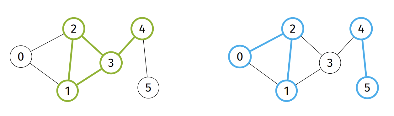
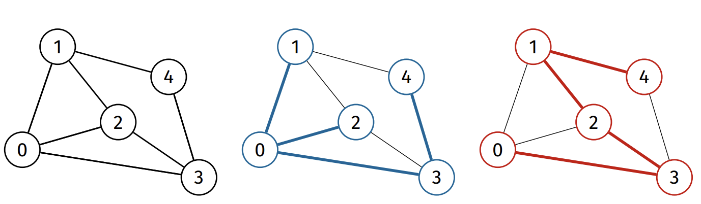
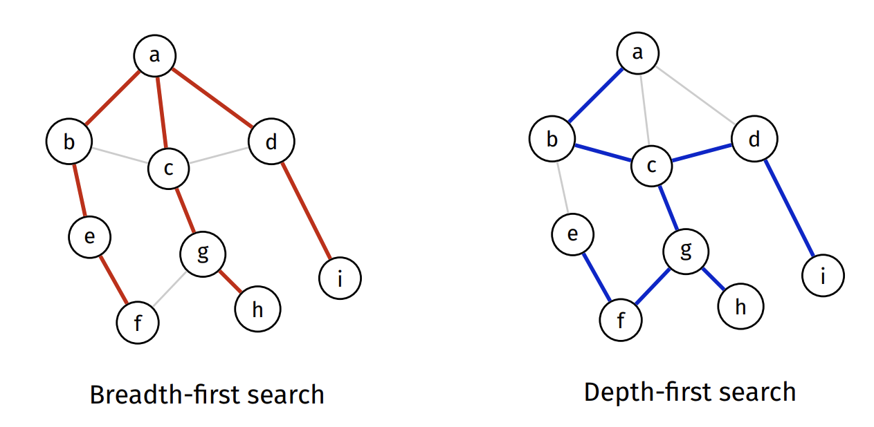
The edges traversed in a graph traversal form a spanning tree.

A traversal starting at vertex ‘a’ forms the following spanning trees:

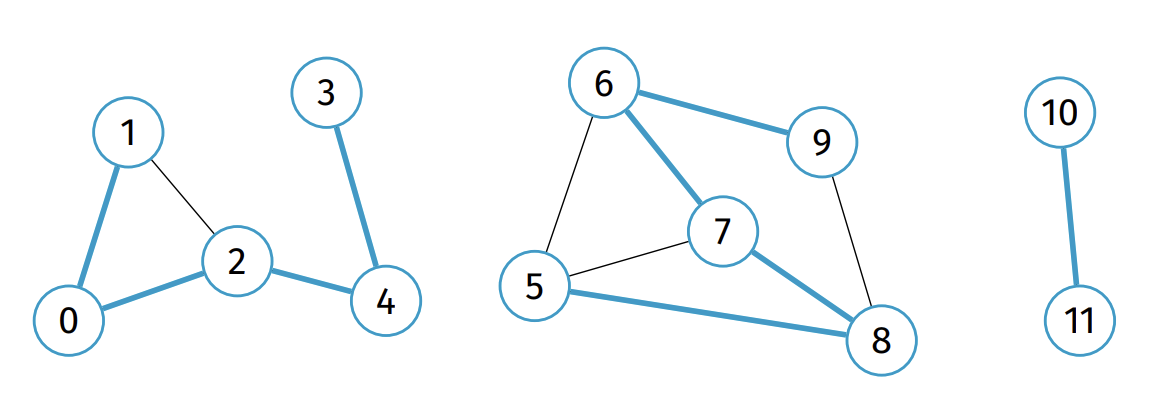
Disconnected Graphs

If a graph is not connected, a graph traversal starting from a given vertex will not traverse the entire graph.

Solution:

After initial traversal is complete, perform traversal again on an unvisited vertex, repeat until all vertices are visited This produces a spanning forest

dfs(G):
  Input: graph G

  create predecessor array, initialised to -1

  for each vertex v in G:
    if predecessor[v] = -1:
      dfsRec(G, v, predecessor)
  ...

Graph Problems

Cycle Checking

A cycle is a path of length > 2 where the start vertex = end vertex and no edge is used more than once.

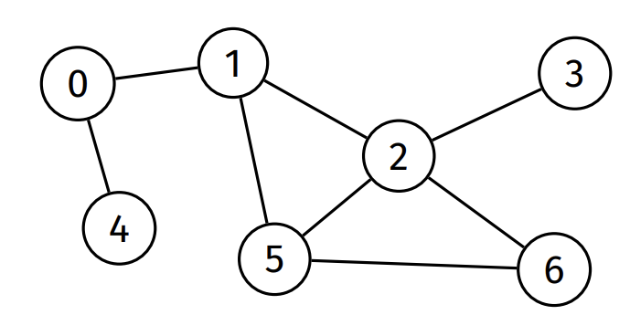
This graph has three distinct cycles:

1-2-5-1, 2-5-6-2, 1-2-6-5-1

Idea to check cycles in a graph:

• Perform a DFS, starting from any vertex
• Keep track of the previous vertex during DFS (to ensure length > 2)
• During the DFS, if the current vertex has an edge to an already-visited vertex, which is not the previous vertex, then there is a cycle
• After the DFS, if any vertex has not yet been visited, perform another DFS, this time starting from that vertex
• Repeat until all vertices have been visited

hasCycle(G):
  Input: graph G
  Output: true if G has a cycle, false  otherwise

  create visited array, initialised to false

  for each vertex v in G:
    if visited[v] = false:
      if dfsHasCycle(G, v, v, visited):
        return true

dfsHasCycle(G, v, prev, visited):
  visited[v] = true

  for each neighbour w of v in G:
    if w = prev:
      continue
    if visited[w] = true:
      return true
    else if dfsHasCycle(G, w, v, visited):
      return true

  return false   

Analysis:

Using adjacency list representation,

• Algorithm is a slight modification of DFS
• A full DFS traversal is $O(V + E)$
• Thus, worst-case time complexity of cycle checking is $O(V + E)$

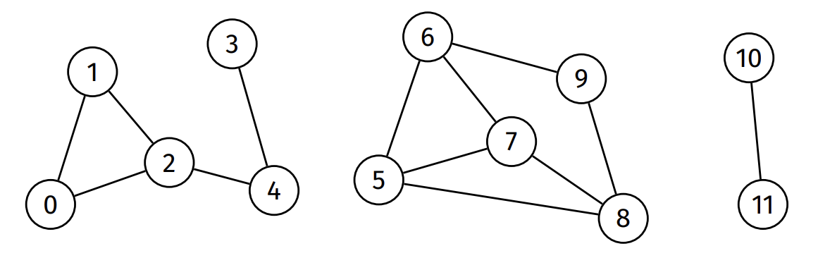
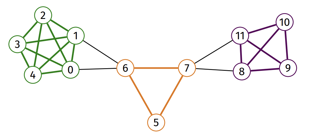
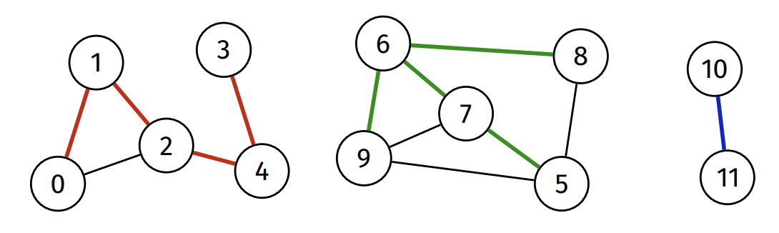
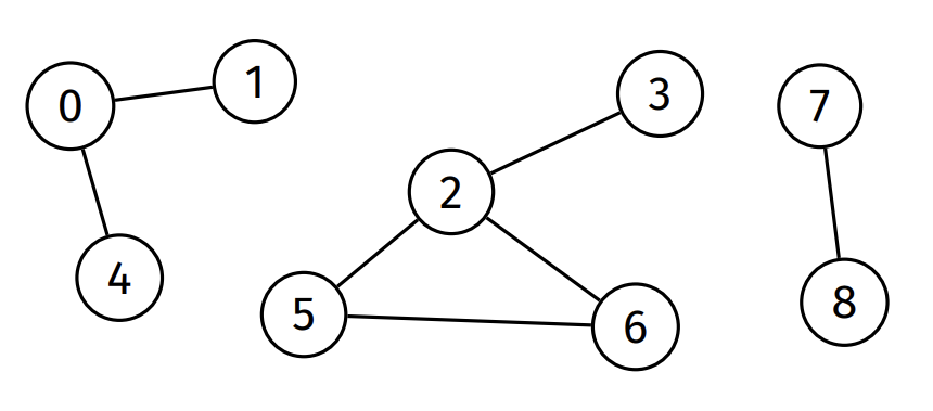
Connected Components

A connected component is a maximally connected subgraph. For example, this graph has three connected components:

Goal:

• Compute an array which indicates which connected component each vertex is in
  • Let this array be called $componentOf$
  • $componentOf[v]$ contains the component number of vertex $v$

Idea:

• Choose a vertex and perform a DFS starting at that vertex
  • During the DFS, assign all vertices visited to component 0
• After the DFS, if any vertex has not been assigned a component, perform a DFS starting at that vertex
  • During this DFS, assign all vertices visited to component 1
• Repeat until all vertices are assigned a component, increasing the component number each time

components(G):
  Input: graph G
  Output: componentOf array

  create componentOf array, initialised to -1

  compNo = 0
  for each vertex v in G:
    if componentOf[v] = -1:
      dfsComponents(G, v, componentOf, compNo)
      compNo = compNo + 1

  return componentOf

dfsComponents(G, v, componentOf, compNo):
  componentOf[v] = compNo
  for each neighbour w of v in G:
    if componentOf[w] = -1:
      dfsComponents(G, w, componentOf, compNo)

Analysis using adjacency list:

• Algorithm performs a full DFS, which is $O(V + E)$

Suppose we frequently need to check:

• How many connected components there are
• Are $v$ and $w$ in the same connected component?
• Is there a path between $v$ and $w$?

Solution is to cache the components array in the graph struct

struct graph {
  ...
  int nC; // number of connected components
  int *cc; // componentOf array
};

However, this information needs to be maintained as the graph changes:

• Inserting an edge may reduce nC
  • If the endpoint vertices were in different components
• Removing an edge may increase nC
  • If the endpoint vertices were in the same component and there is no other path between them

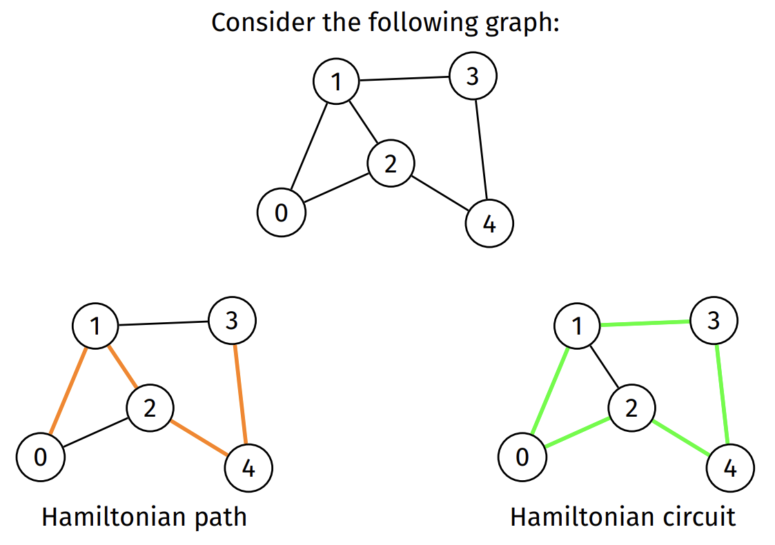
Hamiltonian Path and Circuit

• A Hamiltonian path is a path that includes each vertex exactly once

• A Hamiltonian circuit is a cycle that includes each vertex exactly once

To check if a graph has a Hamiltonian path:

• Brute force
• Use DFS to check all possible paths
  • Recursive DFS is perfect, as it naturally allows backtracking
• Keep track of the number of vertices left to visit
• Stop when this number reaches 0

hasHamiltonianPath(G):
  Input: graph G
  Output: true if G has a has a Hamiltonian path, false otherwise

  create visited array, intialised to false
  for each vertex v in G:
    if dfsHamiltonianPath(G, v, visited, #vertices(G)):
      return true

  return false

dfsHamiltonianPath(G, v, visited, numVerticesLeft):
  visited[v] = true
  numVerticesLeft = numVerticesLeft - 1

  if numVerticesLeft = 0:
    return true

  for each neighbour w of v in G:
    if visited[w] = false:
      if dfsHamiltonianPath(G, w, visited, numVerticesLeft):
        return true

  visited[v] = false
  return false

How to check if a graph has a Hamiltonian circuit:

• Similar approach as Hamiltonian path
• Don’t need to try all starting vertices
• After a Hamiltonian path is found, check if the final vertex is adjacent to the starting vertex

hasHamiltonianCircuit(G):
  Input: graph G
  Output: true if G has a Hamiltonian circuit, false otherwise

  if #vertices(G) < 3:
    return false

  create visited array, initialised to false
  return dfsHamiltonianCircuit(G, 0, visited, #vertices(G))

dfsHamiltonianCircuit(G, v, visited, numVerticesLeft):
  visited[v] = true
  numVerticesLeft = numVerticesLeft - 1

  if numVerticesLeft = 0 and adjacent(G, v, 0):
    return true

  for each neighbour w of v in G:
    if visited[w] = false:
      if dfsHamiltonianCircuit(G, w, visited, numVerticesLeft):
        return true

  visited[v] = false
  return false

Analysis:

• Worst-case time complexity: $O(V!)$
• There are at most V! paths to check ($≈\sqrt{2\pi V}(V/e)^V$ by Stirling’s approximation)
• There is no known polynomial time algorithm

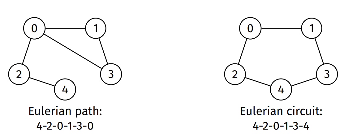
Eulerian Path and Circuit

• An Eulerian path is a path that visits each edge exactly once
• An Eulerian circuit is an Eulerian path that starts and ends at the same vertex

How to check if a graph has an Eulerian path or circuit:

• A graph has an Eulerian path if and only if exactly zero or two vertices have an odd degree, and all vertices with non-zero degree belong to the same connected component
• A graph has an Eulerian circuit if and only if every vertex has even degree, and all vertices with non-zero degree belong to the same connected component

hasEulerianPath(G):
  Input: graph G
  Output: true if G has an Eulerian path, false otherwise

  numOddDegree = 0
  for each vertex v in G:
    if degree(G, v) is odd:
      numOddDegree = numOddDegree + 1

  return (numOddDegree = 0 or numOddDegree = 2) and eulerConnected(G)


hasEulerianCircuit(G):
  Input: graph G
  Output: true if G has an Eulerian circuit
          false otherwise

  for each vertex v in G:
    if degree(G, v) is odd:
      return false

  return eulerConnected(G)


eulerConnected(G):
  Input: graph G
  Output: true if all vertices in G with non-zero degree
          belong to the same connected component
          false otherwise
  
  create visited array, initialised to false

  for each vertex v in G:
    if degree(G, v) > 0:
      dfsRec(G, v, visited)
      break

  for each vertex v in G:
    if degree(G, v) > 0 and visited[v] = false
      return false

  return true

Analysis for adjacency list representation:

• Finding degree of every vertex is $O(V + E)$
• Checking connectivity requires a DFS which is $O(V + E)$
• Therefore, worst-case time complexity is $O(V + E)$

Other Graph Problems

Many graph problems are intractable, that is, there is no known “efficient” algorithm to solve them.

In this context, “efficient” usually means polynomial time.

A tractable problem is one that is known to have a polynomial-time solution.