Introduction

Sorting involves arranging a collection of items in order

Three main cases to consider for input order:

• Random order
• Sorted order
• Reverse-sorted order

When analysing sorting algorithms, we consider:

• $n$: the number of items (hi - lo + 1)
• $C$: the number of comparisons between items
• $S$: the number of times items are swapped

Properties

Properties:

• Stability
  • A stable sort preserves the relative order of items with equal keys.
• Adaptability
  • An adaptive sorting algorithm takes advantage of existing order in its input
  • Allows sorted or nearly-sorted inputs to be sorted much quicker than other inputs (e.g. from O(n log n) to O(n))
  • But, just because a sorting algorith sorts sorted input faster than it sorts random/reverse-sorted input, does not mean that it is adaptive. (Could be O(n log n) on random input, but still O(n log n) on sorted input, but slightly faster)
• In-place
  • Sorts the data within the original structure, without using temporary arrays

Elementary Sorting Algorithms

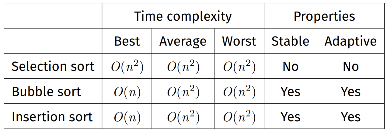
Selection Sort

Method:

• Find the smallest element, swap it with the first element
• Find the second-smallest element, swap it with the second element
• …
• Find the second-largest element, swap it with the second-last element

Time complexity:

Best case: $O(n^2)$
Average case: $O(n^2)$
Worst case: $O(n^2)$

Properties:

Unstable: due to long-range swaps
Non-adaptive: performs same steps, regardless of sortedness of original array
In-place: does not use temporary arrays

Bubble Sort

Method:

• Make multiple passes from left (lo) to right
• On each pass, swap any out-of-order adjacent pairs
• Elements “bubble up” until they meet a larger element
• Stop if there are no swaps during a pass
  • This means the array is sorted

Time complexity:

Best case: $O(n)$ => When array is already sorted, only a single pass required
Average case: $O(n^2)$
Worst case: $O(n^2)$

Properties:

Stable: Swappings are between adjacent elements only
Adaptive: Bubble sort is $O(n^2)$ on average, $O(n)$ if input array is sorted
In-place: does not use temporary arrays

Insertion Sort

Method:

• Take first element and treat as sorted array (of length 1)
• Take next element and insert into sorted part of array so that order is preserved
  • This increases the length of the sorted part by one
• Repeat for remaining elements

Time complexity:

Best case: $O(n)$ => When array is already sorted
Average case: $O(n^2)$
Worst case: $O(n^2)$

Properties:

Stable: Elements are always inserted to the right of any equal elements
Adaptive: Insertion sort is $O(n^2)$ on average, $O(n)$ if input array is sorted
In-place: does not use temporary arrays

Summary of Elementary Sorts

Extra:

Notice that Bubble Sort and Insertion Sort has the exact same properties, so how do we differentiate them? We will test the unknown algorithm with an edge case of sorted elements, but the first and the last elements are swapped (e.g., [n, 2, 3, 4,…, n - 1, 1]). Using this case, bubble sort executes with an O(n^2) complexity, whereas insertion sort is O(n).

Divide-and-Conquer Sorting Algorithms

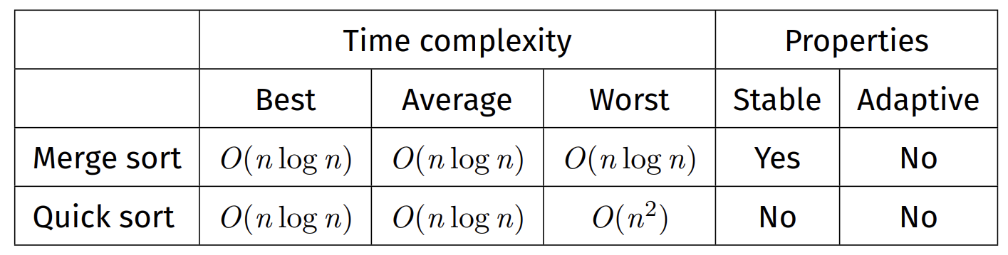
Merge Sort

A divide-and-conquer sorting algorithm:

• split the array into two roughly equal-sized parts
• recursively sort each of the partitions
• merge the two now-sorted partitions into a sorted array

Time complexity:

Best case: $O(n \log n)$
Average case: $O(n \log n)$
Worst case: $O(n \log n)$

Properties:

Stable: Due to taking from left subarray if items are equal during merge
Non-adaptive: Same time complexity for all cases
Not in-place: Merge uses a temporary array of size up to n, and uses $O(\log n)$ stack space.

Sorting a linked list with merge sort uses $O(1)$ extra memory (excluding stack space) since it does not need a temporary array, but simply just rewiring of pointers.

Quick Sort

Method:

1. Choose an item to be a pivot
2. Rearrange (partition) the array so that

• All elements to the left of the pivot are less than (or equal to) the pivot
• All elements to the right of the pivot are greater than (or equal to) the pivot

3. Recursively sort each of the partitions

Partitioning:

• Assume the pivot is stored at index lo
• Create index l to start of array (lo + 1)
• Create index r to end of array (hi)
• Until l and r meet:
  • Increment l until a[l] is greater than pivot
  • Decrement r until a[r] is less than pivot
  • Swap items at indices l and r
• Swap the pivot with index l or l - 1 (depending on the item at index l)

Partitioning is $O(n)$, where n is the number of elements being partitioned

Time complexity:

Best case: $O(n \log n)$ => Choice of pivot gives two equal-sized partitions
Average case: $O(n \log n)$
Worst case: $O(n^2)$ => Bad pivot choice resulting in partitions of size 0 and n − 1 & resulting in n recursive levels

Properties:

Unstable: Due to long-range swaps
Non-adaptive: $O(n \log n)$ average case, sorted input does not improve this
In-place: Partitioning is done in-place, and uses $O(\log n)$ stack space on average (O(n) worst case).

Median-of-Three Partitioning:

Take three values: left-most, middle, right-most.

Pick the median of these three values as our pivot.

Ordered data is no longer a worst-case scenario.

This does not eliminate worst-case of $O(n^2)$, but make it much less likely.

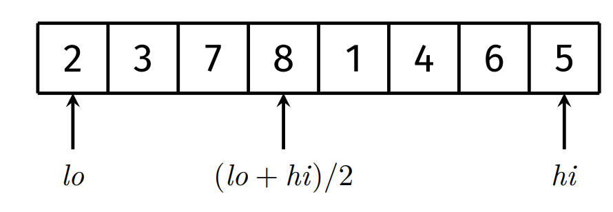
In this example, 5 is chosen as the pivot.

Randomised Partitioning

Pick a random value for the pivot

This makes it nearly impossible to have $O(n^2)$ performance

void randomisedQuickSort(Item items[], int lo, int hi) {
  if (lo >= hi) return;
  swap(items, lo, randint(lo, hi));
  int pivotIndex = partition(items, lo, hi);
  randomisedQuickSort(items, lo, pivotIndex - 1);
  randomisedQuickSort(items, pivotIndex + 1, hi);
}

int randint(int lo, int hi) {
  int i = rand() % (hi - lo + 1);
  return lo + i;
}

Note: rand() is a pseudo-random number generator provided by <stdlib.h>. The generator should be initialised with srand().

Insertion Sort Improvement

For small sequences (when n < 5, say), quick sort is expensive because of the recursion overhead.

Solution: Handle small partitions with insertion sort

#define THRESHOLD 5
void quickSort(Item items[], int lo, int hi) {
  if (hi - lo < THRESHOLD) {
    insertionSort(items, lo, hi);
    return;
  }

  medianOfThree(items, lo, hi);
  int pivotIndex = partition(items, lo, hi);
  quickSort(items, lo, pivotIndex - 1);
  quickSort(items, pivotIndex + 1, hi);
}

Summary of Divide-and-Conquer Sorts

Design of modern cpus mean, for sorting arrays in ram quick sort generally outperforms merge sort

Quick sort is more ‘cache friendly’, good locality of access on arrays

On the other hand, merge sort is readily stable, readily parallel, a good choice for sorting linked lists

Non-Comparison-Based Sorting Algorithms

Radix Sort

Radix sort requires us to be able to decompose our keys into individual symbols (digits, characters, bits, etc.), for example:

• The key 372 is decomposed into (3, 7, 2)
• The key “sydney” is decomposed into (‘s’, ‘y’, ‘d’, ‘n’, ‘e’, ‘y’)

The number of possible symbols is known as the radix, and is denoted by R.

• Numeric: R = 10 (for base 10)
• Alphabetic: R = 26

If the keys have different lengths, pad them with a suitable symbol, for example:

• Numeric: 123, 015, 007
• Alphabetic: “abc”, “zz ”, “t ”

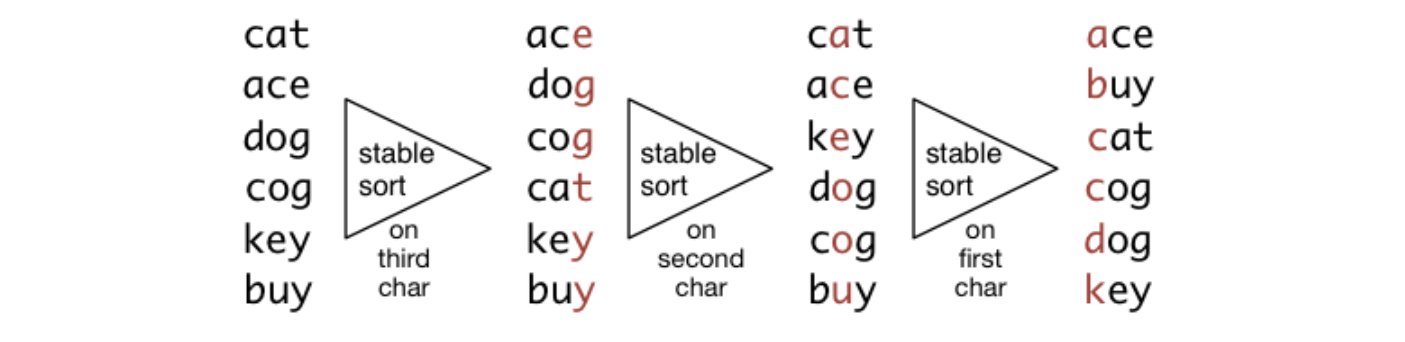
Method:

• Perform stable sort on $k_m$
• Perform stable sort on $k_{m-1}$
• …
• Perform stable sort on $k_1$

Example:

Analysis:

• Array contains $n$ keys
• Each key contains $m$ symbols
• Radix sort uses $R$ buckets
• A single stable sort runs in time $O(n + R)$
• Radix sort uses stable sort $m$ times

Time complexity (best = average = worst) for radix sort is $O(m(n + R))$.

• ≈ $O(mn)$, assuming $R$ is small

Radix sort performs better than comparison-based sorting algorithms:

• When keys are short (i.e., m is small) and arrays are large (i.e., n is large)

Stable: All sub-sorts performed are stable
Non-adaptive: Same steps performed, regardless of sortedness
Not in-place: Uses $O(R + n)$ additional space for buckets and storing keys in buckets